The Binomial distribution

In many cases, it is appropriate to summarize a group of independent observations by the number of observations in the group that represent one of two outcomes. For example, the proportion of individuals in a random sample who support one of two political candidates fits this description. In this case, the statistic ṕ is the count X of voters who support the candidate didivided by the total number of individuals in the group n. This provides an estimate of the parameter p, the proportion of individuals who support the candidate in the entire population.

The binomial distribution describes the behavior of a count variable X if the following conditions apply :

1. The number of observations n is fixed
2. Each observations is independent
3. Each observation represents one of two outcomes ("success" or "failure")
4. The probability of "success" p is the same for each outcome

If these conditions are met, then X has a binomial distribution with parameters n and p, abbreviated B(n,p).

Note : The sampling distribution of a count variable is only well-described by the binomial distribution in cases where the population size is significantly larger than the sample size. As a general rule, the binomial distribution should not be applied to observations from a simple random sample unless the population size is at least 10 times larger than the sample size.

The probability that a random variable X with binomial distribution B(n,p) is equal to the value k, where k = 0, 1 , . . . , n is given by :

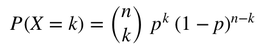
where :

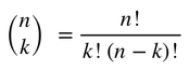
The latter expression is known as the binomial coefficient stated as "n choose k", or the number of possible ways to choose k "successes" from n observations.  For example the number of ways to achieve 2 heads in a set of four tosses is "4 choose 2" or :

Mean and Variance of the binomial distribution

The binomoal distribution for a random variable X with parameters n and p represents the sum of n independent variables Z which may assume the values 0 or 1. If the probability that each Z variable assumes the value 1 is equal to p, then the mean of each variable is equal to 1 x p + 0 x ( 1-p ) = p, and the variance is equal to p ( 1 - p ).  By the addition properties for independent random variables, the mean and variance of the binomial distribution are equal to the sum of the means and variances of the n independent Z variables, so :

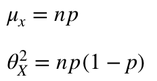
Moreover, for large values of n, the distributions of the count X and the sample proportion ṕ are approximately normal. This result follows from the Central Limit Theorem. The mean and variance for the approximately normal distribution of X are np and np(1-p), identical to the mean and variance of the binomial (n,p) distribution. Similarly, the mean and variance for the approximately normal distribution of the sample proportion are p and p(1-p)/n.