The Word2Vec algorithm

In a word of enhanced connectivity between humans and continuous flow of information, the need for natural language processing (NLP) has now become a key feature of the society of tomorrow. Indeed, in a world where the production and exploitation of ever greater amount of data will become the main source of value, it is now becoming essential to rethink our ways of processing information to be able to adapt to the new paradigm that the 21^st century is offering to us.

In this sense, it appears interesting to analyze the different possibilities that are currently available to automatize information processing and more particularly study the Word2Vec algorithm which truly constitutes the core foundation of the NLP in order to get a deeper knowledge of its inner working and a better understanding of its potential in an era where data is soon to become the new gold.

Plan

1.   Word2Vec history
2. Word2Vec architecture
3. Improvement of the model
4. Main current use & possible future application

1. Word2Vec history

During the past ten years or so, the area of computing science and AI involved in developing the interaction between computer and human in natural language, commonly called NLP, put its focus on trying to adapt the free text produce everyday by our society into numeric values. From this research emerged different two main ideas:

• One hot encoding which is one of the simplest approach possible where each distinct word stands for one dimension of the resulting vector and a binary value indicate whether or not the word is present.

• Word embedding where words and phrases are transformed into vectors of numeric values with much lower and thus denser dimensions.

However, even though the one hot encoding method  seems like a good idea at first, this latter doesn’t take into account contextual information and force us to deal with hundreds of thousands of dimensions which is never a really good idea from a computational standpoint. As such, the commonly used method nowadays is the word embedding one among which we have two main categories :

• Count-based model : unsupervised model based on matrix factorization of a global word co-occurrence matrix. (examples : PCA, topic models, neural probabilistic language models
  

• Context based model : supervised model learning efficient word embedding representation through the prediction of target words. (Word2Vec …)

In this article, we will focus specifically on context based model and more particularly on the Word2Vec model which was a big leap forward in the development of context based model. Indeed, created in 2013 by Tomas Mikolov and its research team at Google, this method was a real milestone allowing for many successful Google applications such as Google translate and others especially with the continuous fine tuning of this algorithm by the team through the implementation of other techniques such as sub-sampling or negative sampling but before going any further into theses specifications let’s see first the basic architecture of this algorithm and how it works under the hood.

2 Word2Vec architecture

As stated before, the Word2Vec model allows us to build predictive models that try to predict a “target” word given its neighbors. However, before going any further in our development we have to choose between two main frames which will define our implementations of the Word2Vec model:

• Continuous Bag of Words (CBOW) : where the words occurring in context (surrounding words) of a selected word are used as inputs to predict the latter

• Skip-Gram where the target word is used to try to predict the words coming before and after it.

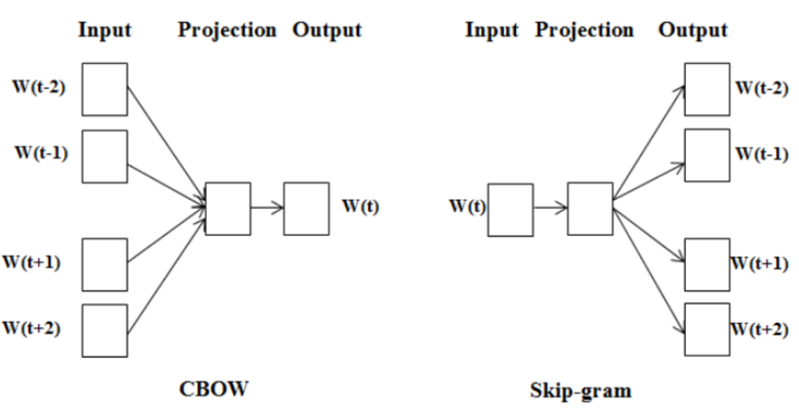
Here we will focus on the Skip-Gram version as it has been proven empirically to give better results. So, now let’s approach the basic architecture of this model.

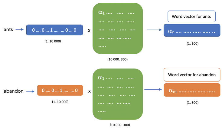
For a better understanding, let’s consider a corpus of 10,000 words, and in this corpus the following couple of words (ants, abandon). The first thing that we’ll do here is to translate each of those two words into a one hot vector (here column matrices of 10,000 rows) as follows :

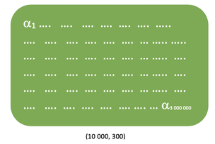
Then following the recommendation from the Google team we’ll use 300 features in order to learn our word vectors and input our couple of words into our network which leads us to end up with a hidden layer represented by a weight matrix of 10,000 rows and 300 columns as shown below:

However due to the fact that we previously transformed our couple of words as one hot vector we can see that the hidden layer will just perform as a lookup table here as shown below :

From this point we then operate a dot product / cosine similarity operation in order to get the similarity between our two word vectors:

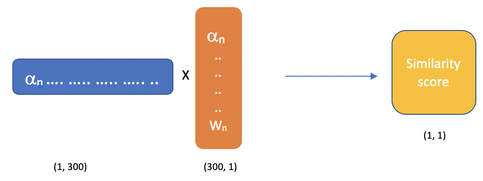
After that, we input our previous similarity score into a sigmoid layer to obtain our output equal to :

• 1 if the word “abandon” is in the context of the target word “ants”

• 0 if the word “abandon” is not in the context of the target word “ants”

Finally, the back-propagation of the errors will work to update the embedding layer to ensure that words which are truly similar to each other have vector such that they return high similarity scores.

Here is another illustration which summarized all the steps that we explain above in a much more broader way:

3 Negative sampling & Subsampling

Negative sampling

Training a neural network means taking a training example and adjusting all of the neuron weight slightly so that it predicts that training sample more accurately. In other word, each training will tweak all of the weights in the network.

Translating that to our corpus of 10,000 words, this means that the tremendous number of weights of our skip-gram model will be slightly updated by every one of our billions of training samples causing serious time processing problem. This is why to avoid this situation we are using what we call negative sampling which will only modify a small percentage of the weights rather than all of them.

How does it work ?

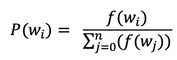
With negative sampling we are going to select a small number of negative words (words for which the network output 0) and only update the weights for those and our context word. However, it is important to note that the negative sample is not randomly selected. Instead, we’re going to use the following variation of the unigram distribution in order to make it more likely for more frequent words to be selective as negative samples :

Subsampling

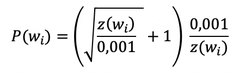
Another problem that we encounter when training our neural network is the one linked to what we can call the common word. Indeed, when looking at the pair (“the”, “car”), the “the” doesn’t tell us much about the meaning of “car” even though it appears in the context of pretty much every word. Also, in the end we will end up with much more sample of “the” that we’ll ideally need to learn a good word vector. This is why, the skip-gram model implements a method called subsampling. This method make it so that for each word we encounter in our training text, there is a chance that we will effectively delete it from the text, the probability being related to the word’s frequency. To compute the probability, the skip-gram model makes use of the following function which has proven empirically to be sufficient in this use case:

Main current use case & possible future applications

Currently the most common use case of the Word2Vec algorithm is mainly translation between languages. However with the growing development of big data and the necessity for big digital companies to always getting a better understanding of their customers to enhance their services, we can say that applications will surely pop up for this NTP model in data analysis and KYC analytics. At last, in a near future with the recent development of the biotech sector and especially of the genetic engineering field, we could imagine that new ways of processing genomic information will be needed and that it could very well become another ground of application for NTP algorithm and Word2Vec in particular.