PCA method

Hi there, hope everyone is doing fine ^^

As we've seen in the previous serie of tutorial on the 7 basic algorithms used in data science, machine learning generally works wonders to build good predictive model on large and concise datasets. However, in most cases the reality is not so simple as we can literally end up with dozens of variables containing inconsistencies and redundant features which at term can become quite problematic given that it usually increase quite dramatically the overall compilation time to the extent that we cannot even compute the model anymore ^^'

Thankfully, different methods exist to decrease the number of features of a given dataset and only retain the most important one and that will be the focus of today's tutorial as we will approach the most commonly used method called Principal Component Analysis (PCA).

So first, what is PCA ?


PCA is a dimensionality reduction technique that enables you to identify correlations and patterns in a data set so that it can be transformed into a data set of significantly lower dimension without loss of any important information. It follows the following 4 steps :

Step 1 : Standardizations of the data
Step 2 : Computing the covariance matrix
Step 3: Calculating the eigenvectors and eigenvalues
Step 4 : Reducing the dimensions of the data set

So let's take a closer look at each of those steps :

Step 1 : Standardizations of the data

Here the idea is to scale our data in such a manner that all the variables and their values lies within a similar range

Exemple :
Let's consider 2 variables in a data set, one with values ranging from 0 to 100 and the second one with values between 1000 and 15000. In such scenario, it appears obvious that the output calculated by using these predictor varibales will be biaised since the variable with a larger will obviously have more impact on the outcome.

That's why it is important to first operate a standardization of our data set in order to avoid the problem of the biaised outcome.

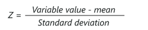
To operate the standardization we simply substract to each value the mean and then divide this result by the overall deviation in the dataset as shown below :

Step 2 : Computing the covariance matrix

In this second step we simply compute the covariance matrix of our data set in order to identify the correlations between our different features.

Quick recap :

• The covariance value denotes how co-dependent two variables are with respect to each other
• If the covariance value is negative, it denotes the respective variables are indirectly proportional to each other.
• A positive covariance denotes that the respective variables are directly proportional to each other.

Step 3: Calculating the eigenvectors and eigenvalues

We calculate the eigenvectors and eigenvalues from our matrix in order to spot where we have the most variance in our data since more variance in the data denotes more information about the said data. Then once we have compute all our eigenvectors and eigenvalues, all we have to do is to sort those by descending orders to get our principal components by order of significance.

Step 4 : Reducing the dimensions of the data set

Once we have all our principal components the last thing that we have to do is to choose the number of principal components that we want to consider in our case and re-arrange our original data with the final principal components representing the most significant information of the dat set. To do so, we multiply the transpose of the original data set by the transpose of the obtained feature vector.

Alright so now that we have a better understandig of how the PCA process works, let's try it for ourselve by implementing it on a real data set with Python.

Application

First thing first let's import the needed libraries :

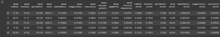
From there, we also import our data and reshape them in order to have a clean dataframe to work with :

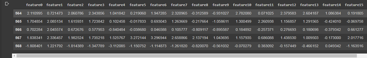
Now, as we discussed before in our presentation of the PCA process we will before doing anything else operate a normalization of our dataset :

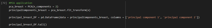
Once it's done, we can easily compute our principal components with the help of the sklearn.decomposition library :

n.b. The choice of principal components here is totally arbitrary so feel free to experiment for yourself !

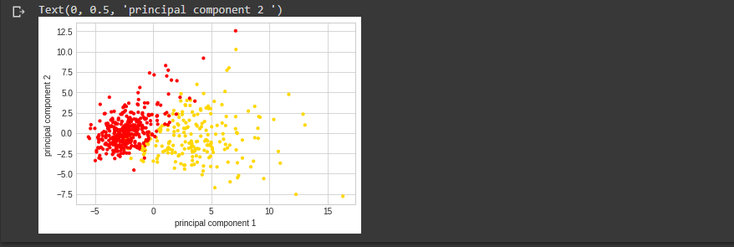
By checking the results here :

we can see that the principal component 1 holds 44.2% of the information while the princpal component 2 holds only 19% of the information meaning that while projecting a thirty dimensional data set onto a two dimensional data set we lost approximately in the 36% of the initial information.

Bonus : Here is the code to plot your results with colab

And that's it for me on the subject of the pCA process ^^. So I hope that you enjoyed this tuto introducing the PCA process and as always don't hesitate to go beyond in order to get a deeper understanding of the notions that we just introduce.

Like always, full code is available here on the github of the website.

I'll catch you on the next one, in the meantime take care and happy coding ✌️