Naives Bayes

Hi there, hope you're doing great ! ^^

In today's tutorial we will approach a machine learning algorithm widely used across multiple applications like spam filtering or classification tasks called the Naive Bayes algorithm.

So as always, at first we will be presenting the theory behind it and illustrate its inner working before going further and implementing it in concrete real life illustrations.

Sounds good ? Well let's start with our theoretical part then ^^

Theory

Given that the naive Bayes algorithm is an extension of the the Bayes Rule based itself on the concept of conditional probability. So before going any further let's do a quick recap of the link between conditional probabilities and the Bayes Rule in order to then be able to understand fully the idea behind the naive Bayes algorithm.

So first, let's go back to the basic and do a quick recap of concept of conditional probability with the help of this following little example.

Consider a school with a total population of 100 persons. These 100 persons can be seen either as Students and Teachers or as a population of 'Males' abd 'Females'.

Given the below tabulation of the 100 people, let's compute the conditional probability that a certain member of the school is a teacher given that he is a man.

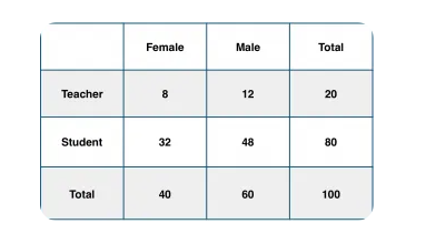
To calculate it we will need to compute the probability that knowing that a certain member of the school is a male, he is also a teacher. In this sense we will need to filter the subpopulation of 60 males and focus on the 12 male teachers among them :

P(teacher | Male) =  P(Teacher & Male ) / P(Male) = 12 / 60 = 0.2

This quick example can be represented as the intersection o fTeacher (A) and Male (B) divided by Male (B). Likewise the conidtional probability of B given A can be computed. The Bayes rule that we use for Naives Bayes, can then be derived from these two notations :

P(A|B) = P(A & B) / P(B)

P(B|A) = P(A & B) / P(A)

So let's see now the Bayes rule. It is first and foremost a way of finding P(Y|X) from P(X|Y) known from the training dataset. To do so we replace A and B in the above formula with the feature X and the response Y.

For observations in test or scoring data, the X would be known while Y is unknown. And for each row of the test dataset we want to compute the probability of Y given the X has already happened.

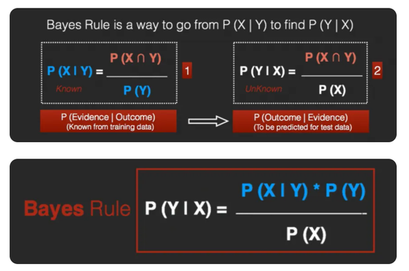
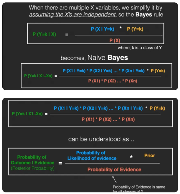
Alright, so the Bayes Rule provides the formula for the probability of Y given X. But in real world problems, we typically have multiple X variables.

=> Thankfully, when the features are independent, we can extend the Bayes Rule to what is called Naive Bayes.

note : It is called "Naive" because of the naive assumption that the X's are independent of each other.

But let's make a quick example to illustrate the functioning of the Naive Bayes algorithm.

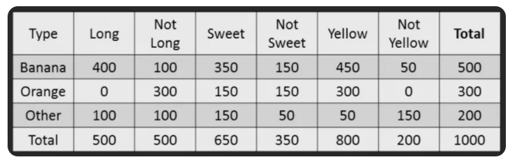
Let's consider we have 1000 fruits which could be either "banana", "orange" or "other".
=> These are the three possible classes of the Y variable.

We also have at our disposal the following X variables, all of which are binary (1 or 0) :

• Long
• Sweet
• Yellow

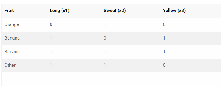
For the sake of simplicity, we will aggregate our training data as to form the accounts table like this :

So our goal here is to predict with the help of our classifier if a given fruit is a "Banana" or "Orange" or "Other" when only the 3 features are known which in other words can be described as trying to predict the Y when only the X variables in the testing data set is known.

But first, let's compute from our training data. Out of 1000 records, we have 500 bananas, 300 oranges and 200 others which gives us :

P(Y = Banana) = 500 / 1000 = 0.5
P(Y= Orange) = 300 / 1000 = 0.3
P(Y= Other) = 200 / 1000 = 0.2

and

P(x1 = Long) = 500 / 1000 = 0.5
P(x2 = Sweet) = 650 / 1000 = 0.65
P(x3 = Yellow) = 800 /1000 = 0.80

Alright, so from there let's compute the probability of likelihood of our 3 features in each case

Probability likelihood for Banana :

P(x1 = Long | Y = Banana ) = 400 / 500 = 0.8

P(x2 = Sweet | Y = Banana) = 350 / 500 = 0.7

P(x3 = Yellow | Y = Banana) = 450 / 500 = 0.9

So the overall probability of Likelihood of evidence for Banana = 0.8 * 0.7 * 0.9 = 0.504.

Then by doing the same for Orange and others we get our respective overall  probability of likelyhood values allowing us as such to use the Naive Bayes theorem as follows :

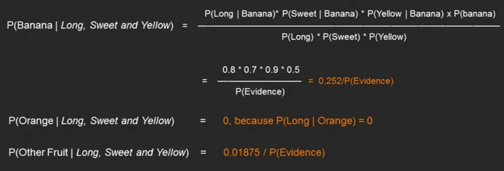
Cleary here, Banana gets the highest probability, so our predicted class in the case where the fruit is Long, Sweet and Yellow will be Banana.


Alright, so now that we have a better understanding of the theory behind the Naive Bayes algorithm and know how to make it work, let's se how we implement it with Python.

Application

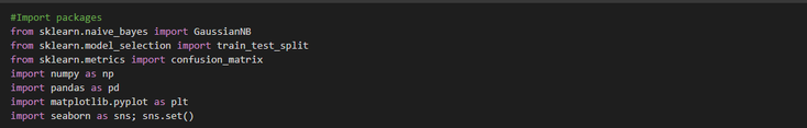
First as always we have to import our packages :

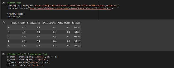
Then we import our data and create our variables for our training and testing datasets :

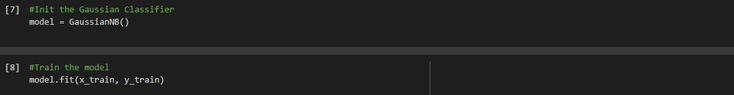
From there we create our model by calling a new instance of the Gaussian classifier object and fit it with our training dataset :

Once it's done we can then predict the output, and plot the score in addition to the confusion matrix of our model :

And that's it we use the naive Bayes algorithm to try to predict the type of Iris that we have depending on the different features that are given to us.

As you can see, it was a pretty quick application just to show you how you can implement it with python and give you a taste of what is possible to do with this algorithm. However, as always don't hesitate to fine tune this example by implementing Laplace correction and so on to try to improve the accuracy of the model.

As always full code can be found here.

I'll see next time, take care ✌️