Logistic Regression

Hi there, welcome in this second tutorial of this serie ^^ Today we're going to stay in the realm of the linear classifier but this time we will put the focus on the Logistic regression. But before firing up python and code anything let's just do a quick recap on what is a logistic regression and how it is working.

Quick overview on the logistic regression

The logistic regression is a fundamental classification technique that belongs to the groupe of linear classifiers. More particularly, it is essentially an easy and fast method for binary classification, although it can also be used for multiclass problems.

As in the previous tutorial on the linear regression, when we're trying to implement the logistic regression of some dependent variable y on the set of independent variables x = (x₁ ,x₂ ,x₃ , ... , x_r ) where r is the number of predictors, we start with the known values of the predictors xi and the corresponding actual response yi for each observation i = 1, ... ,n.

However, here the goal is to find the logistic regression function p(x) such that the predicted responses  p(xi) are as close as possible to the actual response yi for each observation i = 1, ... ,n which in our case are either equal to 0 or 1 given that we're dealing here with a binary classification problem.


Then as usual with linear classifiers, once we have the logistic regression function p(x), we can use it to predict the outputs for new and unseen inputs, assuming that the underlying mathematical dependence is unchanged.

Methodology

Given that the the logistic regression is a linear classifier, we use a linear function f(x) = b₀ + b₁x₁ + ... +  b_tx_t also called the logit. The variables b₀, b₁, ..., bt are the estimators of the regression coefficients, which are also called the predicted weights or just coefficients.

The logistic regression function p(x) is the sigmoid function of f(x) :

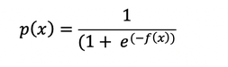
As such it's often close to either 0 or 1. The function p(x) is often interpreted as the predicted probability that the output for a given x is equal to 1. Therefore, 1 - p(x) is the probability that the output is 0.

To fit our model here and obtain the best predicted weights b₀, b₁ , ..., bt we usually use the log-likelihood function (LLF) for all observations i = 1, ...,n. This method called the maximum likelihood estimation is represented by the equation :

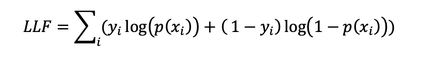
Observations : When y_i = 0 the LLF for the corresponding observation is equal to log(1 - p(x_i)). If p(x_i) is close to y_i = 0 then log(1-p(xi)) drops significantly which is the one thing that we don't want given that our your goal is to obtain the maximum LLF.
 
Once the best weights to define the function p(x) are determined, we can get the predicted outputs p(x_i) for any given input xi. For each observation i = 1, ..., n the predicted output is 1 if p(x_i) > 0.5 and 0 otherwise.

=> The threshold doesn't have to be 0.5, but it usually is.

Classification performance

Binary classification has four possible types of results:

• True negatives : correctly predicted negatives (zeros)
• True positives: correctly predicted positives (ones)
• False negatives: incorrectly predicted negatives (zeros)
• False positives : incorrectly predicted positives (ones)

We usually evaluate the performance of our classifier by comparing the actual and predicted outputs and counting the correct and incorrect predictions.


The different types of logistic regression

There are two main types of logistic regression :

- The single variate logistic regression which is the most straightforward case of logistic regression where we only have one independent variable :

f(x ) = b₀ + b₁x

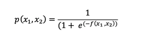
The multivariate logistic regression which has more than one input variable :

f(x₁, x₂) = b₀ + b₁x₁ + b₂x₂

Alright, so now that we have a better understanding of what is the logistic regression let's start using it. To do so, we will do two example, the first being a very basic illustration and the second an example of real life classifier application of handwritten images but enough talking let's get down to it ^^


Application 1

In this first application, we will use the logistic regression in its most simple case and focus on a single-variate binary classification problem.

As in our previous tutorial, we will here use the good general practices reminded below in order to create our classifier :

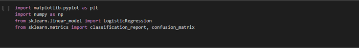
• Import packages, functions and classes
• Get data to work with and if appropriate transform it
• Create a classification model and train it with your existing data
• Evaluate your model to see if its performance is satisfactory

So first thing first, let's open Colab and initiate our code by importing the right libraries :

Then as usual we need to get our data. To this purpose, we create respectively two arrays one for our input x and for our output y :

From here, let's use the LogisticRegression class in order to create and define our classification model and then fit it, in order to determine the value of our coefficients b0, b1, ..., bt giving us the best cost function.

notes : We can easily check the attributes of our model by using the following attributes :

- .classes_
- .intercept_
- .coef_

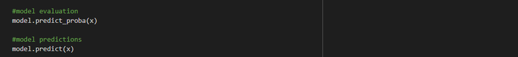
Alright, so now that our model is defined, let's checks its perfomance through the model probability matrix with .predict_proba() and get the actual predictions based on it

From there it's then pretty simple to check the accuracy of the model by using the .score tools calculating the ratio of correct predictions to the number of observation or by using a confusion_matrix if you want more precision :

And that's it for our first example ! ^^

So now that we illustrated simply how to use the logistic regression method on a basic exemple and that we can get a feel of it, let's move on to our second exemple that will be a bot more realistic.

Application 2

here we're going to work on the recognition of handwritten digits. We'll use a dataset with 1797 observations, each of which being an image of a handwritten digit.

=> Each image has 64 px, with a width of 8px and a height of 8px.

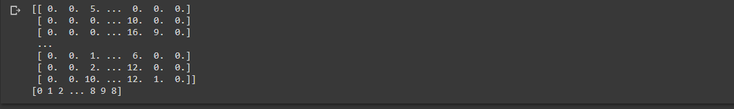
The inputs (x) are vectors with 64 dimensions or values. Each input vector describes one image. Each of the 64 values represents one pixel of the image. The input values are the integers between 0 and 16, depending on the shade of grey for the corresponding pixel.

The output (y) for each observation is an integer between 0 and 9, consistent with the digit on the image. There are ten classes in total, each corresponding to one image.

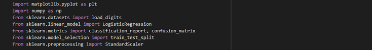
So first let's import the libraries that we need :

Then we import our dataset already pre-uploaded in one of our package:

and split it to create a training and a test set

Also in order to follow the common good practices in use when dealing with linear regression we also here standardize our inputs trhough the use of .fit_transform() allowing us to first fit the instance of StandardScaler to the array passed as the argument, transform this array and returns the new standardized array.

Here, the creation of the model is very similar to what we already did in our previous exemple. The only difference is that we're going to use our train subset to fit the model

Once it's done, come the time of testing our model. To do so,we're going to use our test subset. However, given that we standardized our training input vector x_train, the model that we have is relying on the scaled data, in this sense we have to also scale our test subset.

From then on as you can see below it's pretty straightforward as the steps are exactly similar to what we did before :

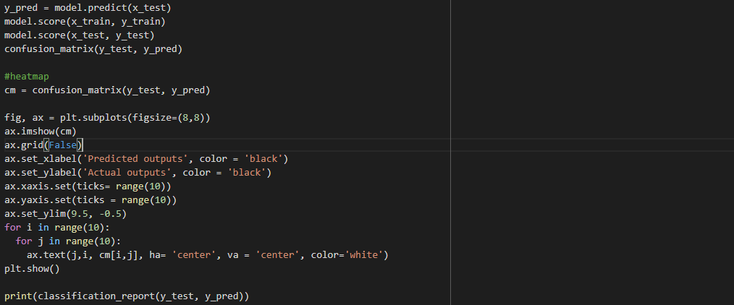
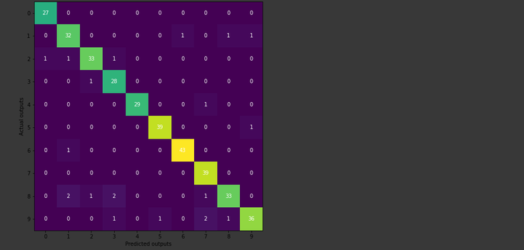
This heatmap illustrates the confusion matrix with numbers and colors. As you can see shades of purple represent small numbers like ( 0,1,2 ) while green and yellow show much larger number.

Moreover, the main diagonal (27, 32,33...) show the number of correct predictions from the test set. For example there are 27 images with zero, 32 images of ones, and so on that are correclty classified.Other numbers correspond to the incorrect predictions. For example, the number 1 in the third row and first column shows that there is one image with the number 2 incorrectly classified as 0.

And that's it for this second application ! ^^ So I hope you enjoy this little tuto on logistic regressions and were able to learn new stuff out of it.

As always full code can be found here.

I'll see you on the next one, in the meantime happy coding ✌️