Linear Regression

Hi there ^^, hope you're doing great !

Today we will start a new serie of tutos in which we will introduce one by one the seven most used algorithms in machine learning.
However, the idea for this serie will not be to jump right into a complex application from a kaggle competition and completly lost ourselves into a massive database ^^'. On the contrary, in this serie we will get back to the basics and see how to use each of those algorithm in addition to presenting the theory at the heart of each of those in order to then take things a bit further in a future follow up serie.

Alright, so let's get down to it and start with our first algorithm : the Linear regression.


So first, what is a regression ?

The regression is a method allowing us to search for relationships among variables. Typically, in regression analysis, we usually consider some phenomenon of interest and registered a number of n observations having each two or more features explaining the observed phenomenon.

For example, we can observe a weather forecast and try to understand how the forecast depends on the temperature, the wind, the atmospheric pressure and so on.

In this case, we will have a regression problem where we will make the presumption that the temperature, the wind and the atmospheric pressure are all independent features impacting at different levels our weather forecast.


Notes :
 
=> The dependant features are called the dependent variables, outputs or responses.

=> The independant features are called the independent variables, inputs or predictors.


Finally regression problems usually have one continuous and umbounded dependent variable while the inputs, on the other hand can be continuous, discrete, or even categorical (gender, nationality, brand...)

 
When do we need it ?

Regressions are useful, to answer whether and how some phenomenon influences an other or how several variables are related. For example, one of the famous use case for regression is the dertmination of house prices in Boston based on differents variables such as the square meter, the number of rooms, the neighbourhood etc. However, this method is also widely used in many different fields such as economy, social sciences, computer science and is a must have to anyone willing to do any serious data analysis.

Linear regression

This type of regression is perhaps the most important and widely used regression techniques due to its simplicity and ease of implementation in most computing language such as Python or R.

In order to implement a linear regression of some dependent variable y on the set of independant variables x = (x1, ..., xr), where r is the number of predictors, we assume a linear relationship between y and x such as :

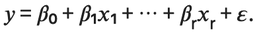
Where :

• β₀, β ₁ , ... , β _R are the regression coefficients
• ε  is the random error

Then with the help of the linear regression, we calculate the estimators of the regression coefficients also called predicted weights, denoted with b₀, b₁, b₂, ..., b_r that define the estimated regression function

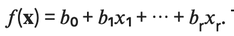
which captures the dependencies between the inputs and the outputs sufficiently well.


The estimated or predicted response f(xi) for each observation i = 1, ..., n should be as close as possible to the corresponding actual response  yi. The differences, yi - f(xi) for all observations i = 1, ... , n are called the residuals. The goal here being to determine the best predicted weights corresponding to the smallest residuals.

=> Usually to get the best weights we minimize the sum of squared residuals (SSR) for all observations i = 1,..., n with the following formula :

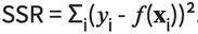
That's what is called the method of ordinary least square.

However, it's important to note that the variation of the actual responses y_i, i = 1, ...,n occurs partly due to the dependence on the predictors but also due to an additional inherent variance of the output. That's why, in order to judge our result we usually use the coefficient of determination denoted R2 specifying which amount of the variation in y can be explained by the dependence on x using the particular regression model.

=> Larger R² indicates a better fit and means that the model can better explain the variation of the output with different inputs.

=> The value R² = 1 corresponds to SSR = 0, that is the perfect fit since the values of the predicted and actual responses fit completely to each other.

 
Now that we have a better idea of what is a linear regression and how to use it, let's start implementing its different version with python ^^

1 Simple Linear regression

This first version of the linear regression is the easiest case possible with a single independant variable y = x.

Note => In this tutorial I will personnaly run the code in Google Colab however, feel free to use whatever python environment you prefer as the code here is basic enough to be usable without any needed change 🙂

Alright, so now let's start coding !

In order to implement our linear regression we will follow 5 basic steps that are good practice and more or less general practice in order to perform properly most regressions:

• Step 1 : Import the packages and classes you need
• Step 2 : Provide data to work with and eventually do appropriate transformations
• Step 3 : Create a regression model and fit it with existing data
• Step 4 : Check the results of model fitting to know whether the model is satisfactory
• Step 5 : Apply the model for predictions

So let's start with our first step and let's import the numpy package and the class LinearRegression from sklearn.linear_model

Once it's done, we need to create a set of data to work with.

⚠️⚠️ Here our inputs should be arrays or similar objects. ⚠️⚠️

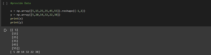
note : We call .reshape() on x as this array is required to be two-dimensional.

Now that we have our data in the right format, it's time to create our model and fit it properly. To do so, we need to to first create a new instance of the class LinearRegression representing the regression model, then fit it by using the existing input and output as the argument to  calculate the optimal values of the weights b0 and b1.

From there, we can get the results to check whether the model works satisfactorily and interpret it by retrieving its coefficient of determination with the help of the .score() function and get the attributes of our model with .intercept_ and .coef_

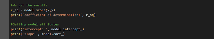
Observation :

We can see here that our b₀ is equal to 5.63 meaning that our model predicts that the response will be 5.63  when x is zero. Moreover, b₁ is equal to 0.54 meaning that the predicted response rise by 0.54 when x is increased by one.

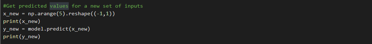
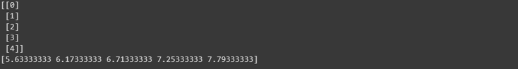
Finally, now that we have a satisfactory model, we can use it for predictions with either existing or new data by using the .predict() function :

Existing values : 

New set of values :

And that's it for the simple linear regression, so let's now move on to our next case.

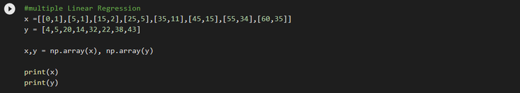
Multiple Linear regression with scikit-learn

Here the first step is similar to the one before :

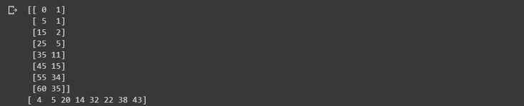
However, our data inputs is modified a bit as in the case of a multiple linear regression our x input must be a two dimensional  array with at least two columns :

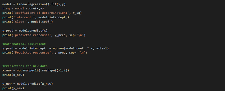
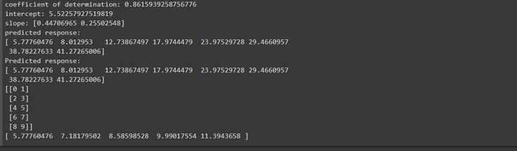
Then all the other steps are unchanged and similar to the case of the simple linear regression as you can see below :

And that's it for the multiple linear regression case, let's now approach our last case.

Polynomial regression

First as usual we import our packages and classes :

=> Here as you can see, we also import the PolynomialFeatures class from sklearn.preprocessing.

Let's now provide our data :

=> Here we will focus on the case where we have :

Consequently, we need here to transform our input data, in order to do our implementation of the polynomial regression. To do so, we are going to use the class PolynomialFeatures to transform our input array x and allow it to contain the additional column with the values of x².

So first let's create a new instance of the PolynomialFeature class with the right arguments :

⚠️⚠️ Important ⚠️⚠️ Before being able to apply our transformer to our input data we need to fit it with those :

Once it's done, our transformer is now ready to create a new, modified input as follows :

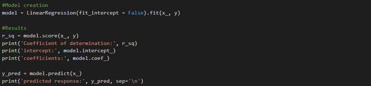
From that point on, the following steps are identical to those in our previous linear regressions, at the minor difference that here we're working with the modified input x_ :

Bonus 1  

You can also implement linear regression in Python by using the package statsmodels. Typically, this is desirable when there is a need for more detailed results.

As before the first step is to import packages :

Then we provide our data

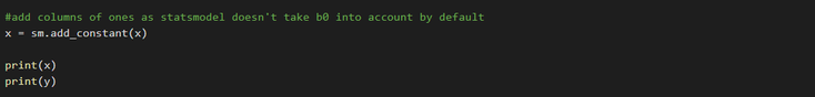
However it's a bit tricky here because this package doesn't take b0 into account by default so we need to add it manually to our input as follows :

the regression model based on ordinary least squares is an instance of the class statsmodels.regression.linear_model_OLS and is obtain as follows :

⚠️⚠️ The first argument here is the output followed with the input ⚠️⚠️

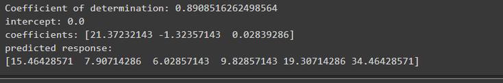
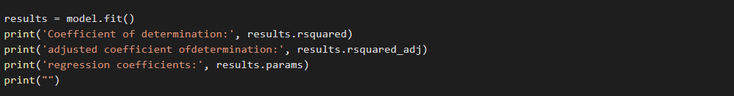
Once the model is created we fit it and then use the .summary() function in order to the table with the results of our linear regression.

To then obtain predicted response on our input values used to create the models we have the choice between two function .fittedvalues() or .predict() :

Bonus 2

You can find on this github page an additional file where all those regressions are put into ready to use functions.

And that's it for today !

So as always don't hesitate to play around with those functions and classes to get a deeper understanding and try it out for yourself on different sets of data.


The full code for this tuto can be found here.

See you on the next one, take care ✌️