CART Algorithm

Hi there, hope you're doing great ^^

In this third tuto we will leave aside linear regression to focus on decision tree algorithm and more particularly on the Classification and Regression Tree also called CART. But before trying to implement it with Python as always let's dive a bit in the theory behind it in order to understand a bit better what we're dealing with here.

Theory

A decision tree is a flowchart-like tree structure where an internal node represents feature, the branch represents a decision rule and each leaf node represents the outcome. The topmost node in a decision tree is known as the root node and the goal here is to make the algorithm learn to partition recursively on the basis of the attribute value.

How does it work ?

The basic idea behind any decision tree algorithm is as follows :

• Select the best attribute using Attribute Selection Measures to split the records (Here given that we focus on the CART  algorithm we will use exclusively the Gini Index
  
• Make that attribute a decision node and break the dataset into smaller subsets.
• Starts tree building by repeating this process recursively for ach child until one of the following condition appears :

1. All the tuples belong to the same attribute value
2. There are no more remaining attributes
3. There are no more instances

In order to make things easier to understand for each an everyone let's do a quick example :

Let's consider the following dataset of 14 instances of golf playing decisions based on outlook, temperature, humidity and wind factors.

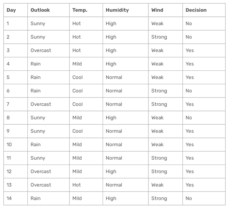
The idea here is to build our decision tree with the help of the Gini index.

Quick recap  :

The GINI index which is the metric for classification task in CART sores the sum of squared probabilities of each class an is calculated as follows :

GINI = 1 - Somme(Pi)^2 for i = 1 to number of classes

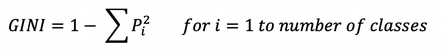
So let's calculate our GINI index for each our nominale features.

In the case of the Outlook, it can be sunny, overcast or rain.

So we obtain :

Gini(outlook = Sunny) = 1 - (2/5)^2 - (3/5)^2 = 1 - 0.16 -0.36 = 0.48

Gini(Outlook = Overcast) = 1 -(4/4)^2 - (0/4)^2 = 0

Gini(Outlook = Rain) = 1 -(3/5)^2 -(2/5)^2 = 1 - 0.36 -0.16 = 0.48

Let's now calculate the weighted sum of our gini indexes for the Outlook feature :

Gini(Outlook) = (5/14) *0.48 + (4/14) *0 + (5/14)*0.48 = 0.171 + 0 +0.171 = 0.342


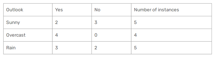
Let's focus now on the Temperature. Here we have 3 different values : Cool, Hot and Mild :

In this case we have :

Gini(Temp = Hot) = 1 - (2/4)^2 - (2/4)^2 = 1 - 0.25 - 0.25 = 0.5

Gini(Temp = Cool) = 1 - (3/4)^2 - (1/4)^2 = 1 - 0.5625 - 0.0625 = 0.375

Gini(Temp= Mild) = 1 - (4/6)^2 - (2/6)^2 = 1 - 0.444 - 0.111 = 0.445

and :

Gini(Temp) = (4/14) * 0.5 + (4/14) * 0.375 + (6/14) * 0.445 = 0.142 + 0.107 + 0.190 = 0.439
 

Let's do the case for Humidity :

Here humidity is a binary class feature and can only be high or normal.

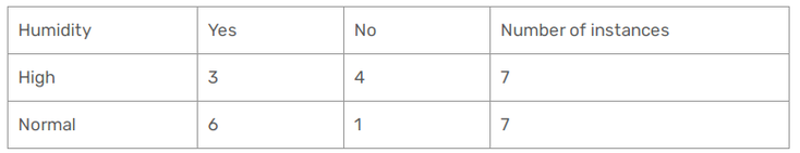
Gini(Humidity = High) = 1 - (3/7)^2 - (4/7)^2 = 1 - 0.183 - 0.326 = 0.489
Gini(Humidity = Normal) = 1 - (6/7)^2 - (1/7)^2 = 1 -0.734 -0.02 = 0.244

Gini(Humidity) = (7/14)*0.489 + (7/14)*0.244 = 0.367

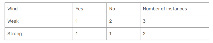
Finally let's see the case of the Wind. Here it is also a binary class and it can be either weak or strong :

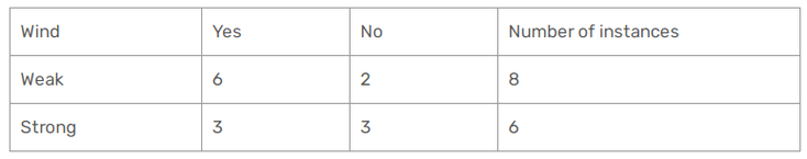
Gini(Wind = Weak) = 1 - (6/8)^2 - (2/8)^2 = 1 - 0.5625 - 0.062 = 0.375
Gini(Wind = Strong) = 1 - (3/6)^2 - (3/6)^2 = 1 - 0.25 - 0.25 = 0.5
Gini(Wind) = (8/14) * 0.375 + (6/14) *0.5 = 0.428


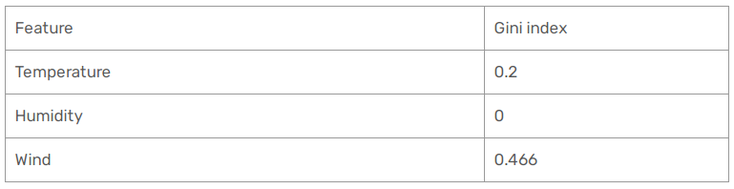
Alright, so now that we have our Gini index for each of our feature, let's compare it and choose the one that costs the lowest :

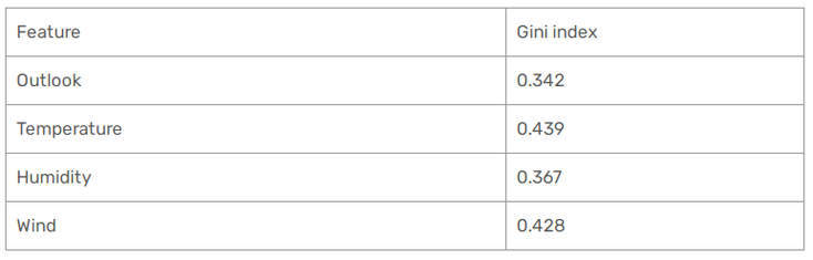
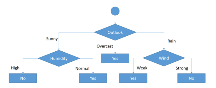
Here, it's outlook so we'll put it at the top of the tree

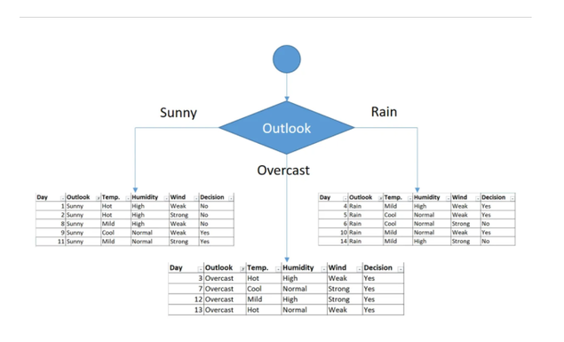
Furthermore in this particular case, you can spot that in the case where the Outlook is "overcast" the decision is always Yes. So we can deduct that the overcast leaf is over.

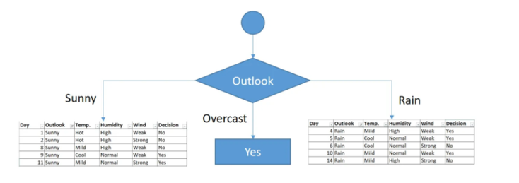
Alright, so now let's focus on the sunny outlook :

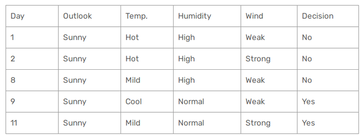
As before let's calculate the Gini index for our lasting features :

Gini of Temperature for sunny outlook

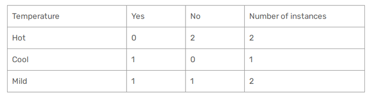
Gini(outlook = Sunny and Temp = Hot) = 1 - (0/2)^2 - (2/2)^2 = 0

Gini(Outlook = Sunny and Temp = Cool) = 1 -(1/1)^2 - (0/1)^2 = 0

Gini(Outlook = Sunny and Temp = Mild) = 1 -(1/2)^2 - (1/2)^2 = 0.5


Gini(Outlook = Sunny and Temp) = (2/5) *0 + (1/5) *0 + (2/5)*0.5 = 0.2


Gini of Humidity for sunny outlook

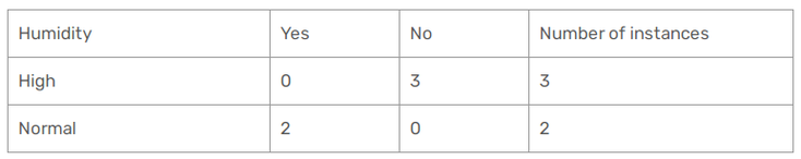
Gini(outlook = Sunny and Humidity = High) = 1 - (0/3)^2 - (3/3)^2 = 0

Gini(Outlook = Sunny and Humidity = Normal) = 1 -(2/2)^2 - (0/2)^2 = 0

Gini(Outlook = Sunny and Temp) = (3/5) *0 + (2/5)*0.5 = 0

Gini of Wind for sunny outlook

Gini(outlook = Sunny and Wind = Weak) = 1 - (1/3)^2 - (2/3)^2 = 0.266

Gini(Outlook = Sunny and Wind = Strong) = 1 -(1/2)^2 - (1/2)^2 = 0.2

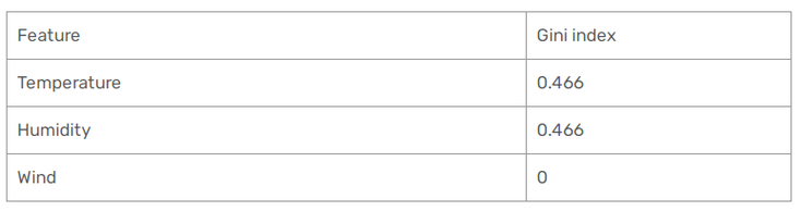
Gini(Outlook = Sunny and Wind) = (3/5) *0.266 + (2/5)*0.2 = 0.466

So we obtain the following results :

and as such choose the humidty feature here :

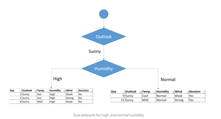
From there you can spot that the decision is always negative for the combination of high humidity and sunny outlook so we can conclude that the branch is over.

Alright, now let's finally focus on the Outlook rain :

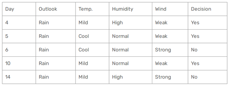
Let's calculate our Gini index for our different cases :

Gini of Temperature for rain outlook

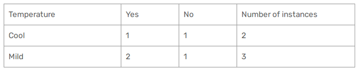
Gini(outlook = Rain and Temp = Cool) = 1 - (1/2)^2 - (1/2)^2 = 0.5

Gini(Outlook = Rain and Temp = Mild) = 1 -(2/3)^2 - (1/3)^2 = 0.444

Gini(Outlook = Rain and Temp) = (2/5) *0.5 + (3/5) *0.444 = 0.466

Gini of Humidity for rain outlook

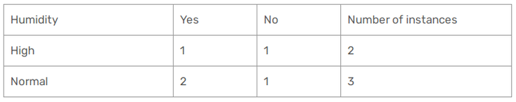
Gini(outlook = Rain and HUmidity = High) = 1 - (1/2)^2 - (1/2)^2 = 0.5

Gini(Outlook = Rain and Humidity = Normal) = 1 -(2/3)^2 - (1/3)^2 = 0.444

Gini(Outlook = Rain and Humidity) = (2/5) *0.5 + (3/5) *0.444 = 0.466

Gini of Wind for rain outlook

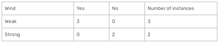
Gini(outlook = Rain and Wind = Weak) = 1 - (3/3)^2 - (0/3)^2 = 0

Gini(Outlook = Rain and Wind = Strong) = 1 -(0/2)^2 - (2/2)^2 = 0

Gini(Outlook = Rain and Wind) = 0

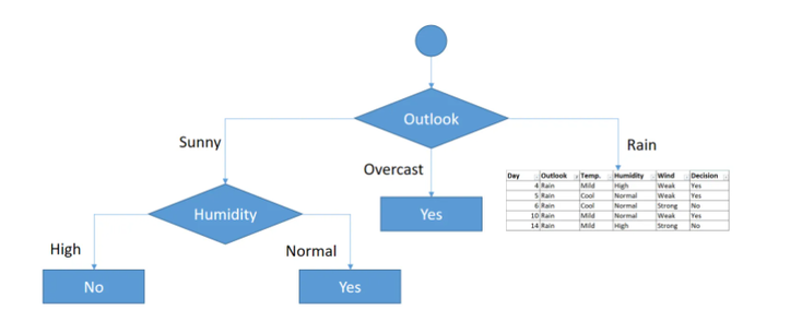
We end up with the following results :

And accordingly choose the wind feature.

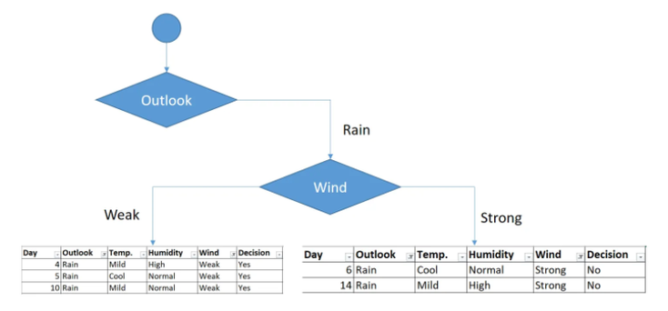
Also here we can see that when the Wind is Weak the decision is always Yes and that the wind is strong the decision is always negative so we can deduct the following :

And that's how the building process of a decision tree using Cart is working. So now that we understand the theoretical part let's see how we can implement that using python.

Application

To implement the CART algorithm with Python, we will create a decisional tree based on the Pima Indians Diabets database in order to predict whether or not a patient has diabetes based on certain diagnostic measurements in the dataset. (for more information see here : https://www.kaggle.com/uciml/pima-indians-diabetes-database)

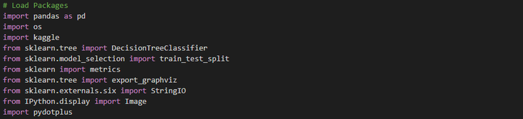
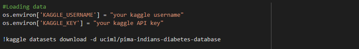
So first thing first open Colab and let's import the following packages :

Once it's done let's download the dataset on which we will work for this application.

Note : I'm using Colab here to perform this tuto, however if you're not and prefer to use another IDE here is a link to the dataset.

Alright, so once our data are downloaded, let's reformat them a bit in order to have something cleaner to work with :

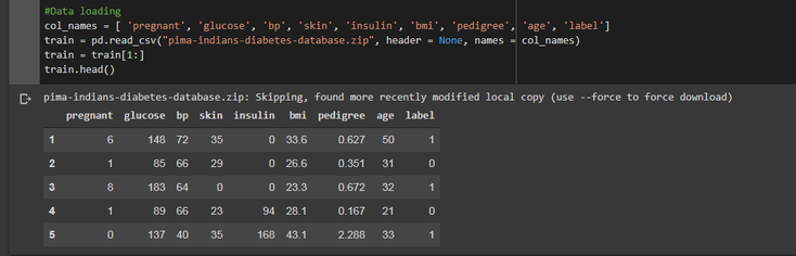
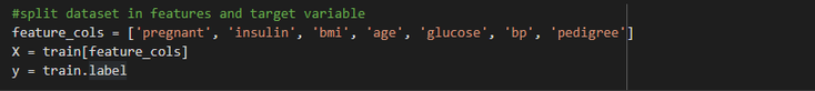
and split them into a training and a test set :

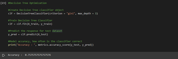
Alright so now that we're set as in the linear regression case in order to create our tree we have to instantiate a new tree classifier object, fit it with our training dataset and measure it's accuracy by confronting it with our test dataset :

Now the only thing left is to print out the graph of our decisional tree with the help of pydotplus :

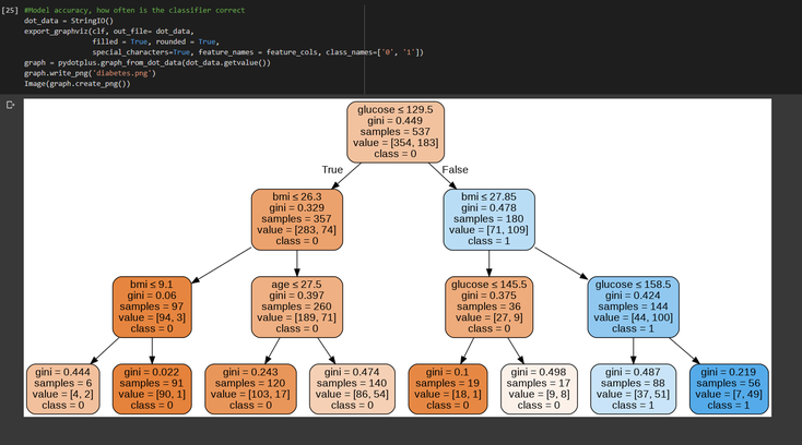
And that's it we successfully implemented a basic specification of the CART model to create a classifier on our Pima Indians Diabets database predicting the class of each patient depending on several independant variables such as bmi, age etc.

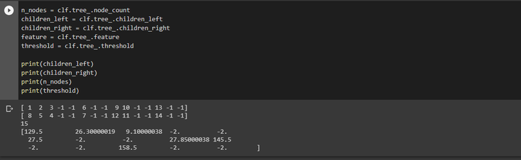
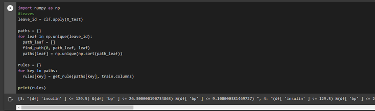
Bonus : From there we can also extract the 8 decision tree rules of our tree. To do so, first we need to get information about the tree that was constructed.

Explanation of the results :

The children left correspond to all the children node of class 0 allowing us to attain the leaf of class 0, as you can see if we follow the rule number 1 :

glucose < 129.5 => bmi < 26.3 => bmi< 9.1 on the fourth and fifth cells we reach the bottom of our tree where Gini = 0.444 and 0.022 respectively.

That's why we have [1, 2, 3, -1 , -1 , ...]

The children right is the exact same thing but in the case where the class is equal to 1.

The thresholds are the ones that are specified on our previous graph.


Once we have those informations, we define two recursive functions. The first one to find the path from the tree's root to create a specific node (all the leaves in our case). The second one to write the specific rules used to create a node given its creation path.

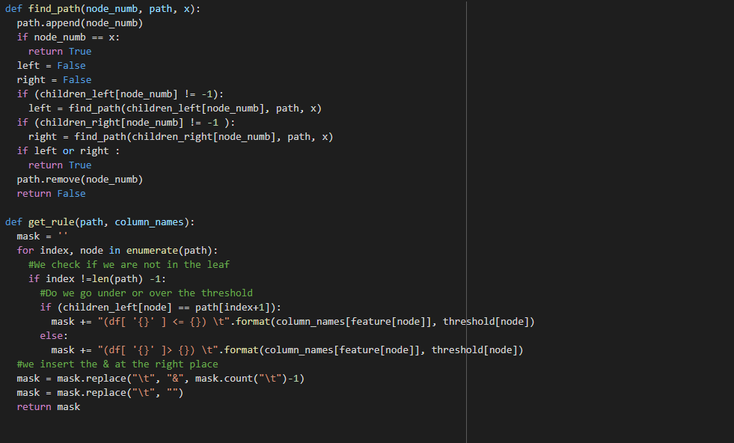
Finally we use those two functions to first store the creation path of each leaf and then store the rules used to create each leaf.

So congrats if you made it up to this point and even made the extra mile to also do the bonus part and as always I'll let you play around with it in order for you to get a deeper understanding of it by for example trying to explore other tree algorithms or else.

As always, full code can be found here.

See you on the next tuto and in the meantime happy coding ✌️