Quick analysis of the Buy & Hold strategy

Hi everyone !  😃

Today we're gonna make a quick analysis of the infamous Buy & Hold strategy but instead of using python we will this time use excel and more specifically VBA to change a little bit and understand how you can easily perform a basic portfolio analysis without having to come down with a sledgehammer. 

Ready ? Let's code then ! 🖥

1 What is VBA and how to set it up ?

If you're already know what is VBA you might want to skip this part as I will just quickly recap what is VBA and how to set it up quickly and nicely on your computer. So if you're still here, don't worry setting up VBA is quite simple and can be done in a matter of minutes but first thing first let's define what is VBA.

VBA or Visual Basic for Application is an integrated implementation of Microsoft Visual Basic which allows you to create your own macro by directly coding them. In other words, it is the tool that allows you to develop programs that control Excel as well as the other members of the Office family.

Now, let's see how you unlock vba on your excel and follows those steps :

1.  Click File
2.  Click Options
3.  Click Customize Ribbon
4.  Under the list of Main Tabs, select Developer
5.  Click OK

The developer is now normaly appearing on the Ribbon and from it you can open the Visual Basic Editor or else you can also the short cut Alt + F11 to be automatically redirect to the VBA editor.

2 Data and methodology

In this tuto, our aim is to perform a quick analysis of a Buy & Hold portfolio. in this sense, we're not gonna do anything crazy and simply consider on the period 2015-12-31 - 2018-10-04  an initial investment of 100 000$ in a portfolio with the following distribution : 

• 20% Apple ( AAPL )
• 10% Amazon ( AMZN )
• 5% Biogen Inc ( BIIB )
• 10% Facebook ( FB )
• 10% Google ( GOOGL )
• 20% Microsoft ( MSFT )
• 5% Netflix ( NFLX )
• 15% Qualcomm ( QCOM )
• 5% Tesla ( TSLA )

Then in order to analyze this portfolio we will compute :

• it's variance and standard deviation
• the historical Value at Risk (VaR) 95%
• the alpha and beta of our portfolio
• a graphical representation of the portfolio returns distribution on the period
• the Simple Moving Average 20 (SMA 20) just to play around and see what's the mechanism behind the rolling python function that we used in this previous tuto

3 The code

( Note : In the following I decided to code with the cells and to not use variables in order to be a little bit more clear inwhat I do but a good exercise could be to change the code by using some variables in order to clean it up a little bit. )

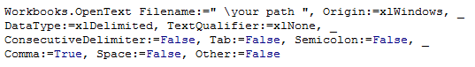
Before starting to compute our different indicators, we have to download our data (click here ). However, as you cann see those data that were extract from yahoo finance are under the csv format, hence we have to first reshape them in accordance to the excel format:

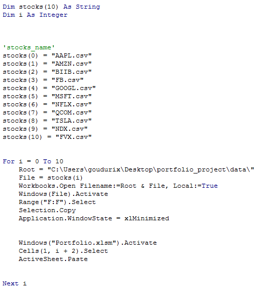
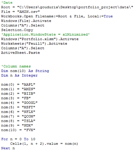
Once, all our files are correctly reshaped we have to call them into our main workbook in order to be able to work with them. However, we will only call the adjusted prices as it is with those that we will work.

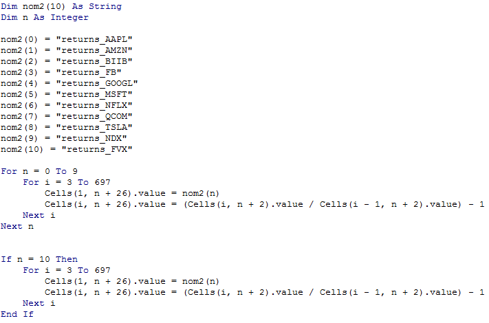
Now that we have load the adjusted prices for stocks on the period we can easily compute their respective daily returns as follows by using two For loop.

Note : Here I chose to use a mix of For and If loop in the case of the risk free rate FVX just to show that it is also possible to use a For loop inside a If loop however don't hesitate to modify the code in order to get rid of it and use only the first For loop.

From there, as you may have already guess we can easily compute the daily returns of our portfolio on the second Sheets in my case 'Feuil2' as follows :

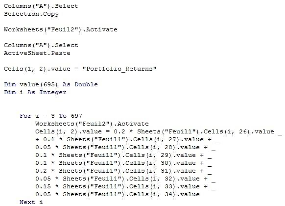
And here we can say that we pretty much have done the hardest part of the work which was to clean our data an get a workable column representing our portfolio daily returns.

Now let's get down to our indicators and compute them !

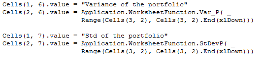
First on our list are the variance and standard deviation and as you may know excel already has functions to compute those so let's call them :

Now moving to the historical Value at Risk we can see that once again, we already have a formula in excel to deal with its calculation so the only thing to do here is to specify the righ percentile as follows :

For the computing of the beta and of the alpha of our porfolio however we'll need to make some extra steps. Let's start with the beta as you know the beta of a portfolio is defined as :

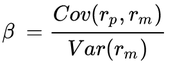
with :

rp the portfolio return

rm the market return

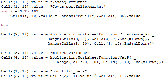
Here as all those stocks are quoted on the Nasdaq we will assume that the market is the Nasdaq.  Now all we have to do is to compute the covariance between the returns of the market and of our portfolio and divide it by the variance of the market :

We now continue with the alpha. As we know the formula to compute the alpha of a portoflio is  :

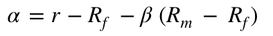
with :

• r : the security’s or portfolio’s return
• R_f  = the risk-free rate of return
• beta = systemic risk of a portfolio (the security’s or portfolio’s price volatility relative to the overall market)
• R_m  = the market return

Note : here we will consider the treasury yield 5 years as our risk free rate

So in our case to compute our alpha we will need to code the above if we want to obtain our alpha for the overall period :  

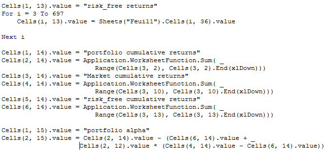
And that's it  ! We have make a quick analysis of our portfolio with the help of the usual indicators ( var, std, VaR ... )

Now let's go a little bit further and see how we can get the SMA20 and make a graphical representation the distribution of our portfolio returns. 

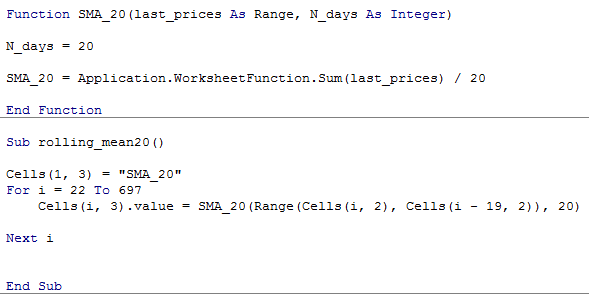
First let's see the SMA 20. As you know the SMA is an arithmetic moving average calculated by adding recent closing prices and then dividing it by the number of time periods in the calculation average. So in our case we will have to compute the mean on the last 20 days for each day of our period which can be easily perform with the help of a For loop  :

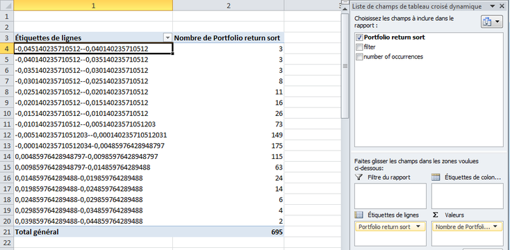
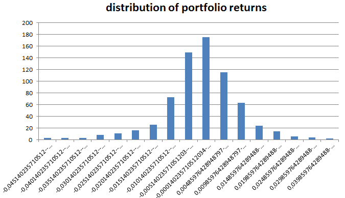
Finally let's see how we can make our graphical representation for the distribution of our portfolio returns. First we need to sort our returns in order to then use them as our dataset.

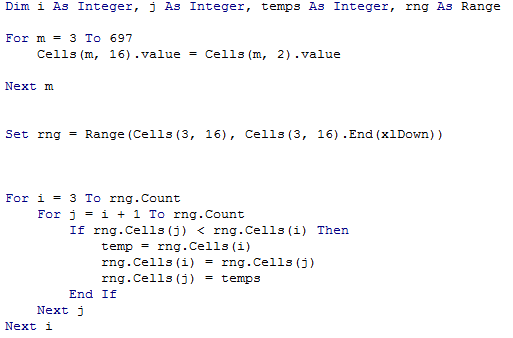
Once we've done that, we create a pivot table as below and use its data to create our graph :

And that's it we're done ! 🙂

As always you'll find the full code here and don't hesitate to play along with the pivot table or clean a little bit this graph by changing the X-axis and so on.

See y'all !